CS134 Project Final Report
A Machine
Learning System for Stock Market Forecasting
My email: Jianfeng.Huo@dartmouth.edu
Abstract
Support vector machines (SVMs) are
promising methods for the prediction of financial time series. This project
applies SVMs to predict the stock price index. In addition the project examines
the feasibility of applying SVM in financial forecasting by comparing it with
traditional linear regression method. The experimental results show that SVM
provides a promising alternative to stock market prediction. What is more I
made an experiment to test the sensitivity of SVMs to some of the parameters.
Introduction/ Background
Recently,
a large amount of amazing work has been done in the area of analyzing and
predicting stock prices and index changes using Machine Learning Algorithms.
Intelligent Trading Systems has been used for most of the stock traders to help
them in predicting prices based on various situations and conditions, thereby
helping them in making instantaneous investment decisions. Stock market prediction
is regarded as one of the most challenging task in financial time-series
forecasting. This is primarily because the underlying nature of the uncertain
financial domain and in part because of the mix of known parameters (Previous
Day’s Closing Price, P/E Ratio etc.) and unknown factors (Election Results,
Rumors etc.).
In
the last few years, significant progress has been made for the stock market
forecasting through the use of SVMs. SVMs were first used by Tay & Cao for financial time series forecasting [1].
Kim has proposed an algorithm to predict the stock market direction by using
technical analysis indicators as input to SVMs [6]. Studies have compared SVM
with Back Propagation Neural Networks (BPN). The experimental results showed
that SVM outperformed BPN most often though there are some markets for which
BPN have been found to be better [7]. These results may be attributable to the
fact that the SVM implements the structural risk minimization principle and
this leads to better generalization than Neural Networks, which implement the
empirical risk minimization principle.
In my project, I will implement a machine learning
system which is proposed by Lijuan Cao and Francis
E.H. Tay [1] based on Support Vector Machines (SVMs) for
stock market prediction. The prime goal of the project is: given a series of
previous days’ stock market indices I can predict the indices of the following
days. Figure 1 show the input and output of my proposed system:
Figure
1 Input and Output of the system
Method
The SV
machine was developed at AT&T Bell Laboratories by Vapnik and coworkers. It
was first applied to the classification problems. Within a short period of
time, SV classifiers became competitive with the best available systems for
both OCR and object recognition tasks. In
this case we try to find an optimal hyperplane that separates two classes. In
order to find an optimal hyper plane, we need to minimize the norm of the
vector w, which defines the separating hyper plane. This is equivalent
to maximizing the margin between two classes. Recently with the introduction of
ε-insensitive loss function, SVMs has been extended to solve non-linear
repression problems. In the case of regression, the goal is to construct a hyperplane
that lies "close" to as many of the data points as possible.
Therefore, the objective is to choose a hyperplane with small norm while
simultaneously minimizing the sum of the distances from the data points to the
hyperplane. Both in classification and regression, we obtain a quadratic
programming problem where the number of variables is equal to the number of
observations [4].
Regression
approximation emphasizes the problem of estimating a function based on a given
set of data ![]() (xi is the input vector and di is the desired
value), which is produced from the unknown function. SVMs approximate the
function in the following form:
(xi is the input vector and di is the desired
value), which is produced from the unknown function. SVMs approximate the
function in the following form:
Where
![]() are the features of inputs
and
are the features of inputs
and ![]() , b are coefficients. Thus they are estimated by minimizing the
regularized risk function (2):
, b are coefficients. Thus they are estimated by minimizing the
regularized risk function (2):
In
equation (2), the first term ![]() is the ε-insensitive loss function.
It is a self-explanatory function that indicates the fact that it does not
penalize errors below ε. The second term
is the ε-insensitive loss function.
It is a self-explanatory function that indicates the fact that it does not
penalize errors below ε. The second term ![]() is used as a measure of
function smoothness. C is a prescribed constant representing determining the
trade-off between the training error and model smoothness. Introduce slack
variables ζ, ζ* to the above equations we have the following
constrained function:
is used as a measure of
function smoothness. C is a prescribed constant representing determining the
trade-off between the training error and model smoothness. Introduce slack
variables ζ, ζ* to the above equations we have the following
constrained function:
Minimize:
Subject to:
![]()
![]()
![]()
Figure 2 depicts the situation graphically. Only the points outside the
shaded region contribute to the cost insofar, as the deviations are penalized
in a linear fashion.
Figure
2 the soft margin loss setting corresponds for a linear SV machine
Thus,
Eq. (1) becomes the following explicit form:
Lagrange
Multipliers
In
function (5), ![]() are the Lagrange multipliers introduced.
They satisfy the
are the Lagrange multipliers introduced.
They satisfy the ![]() equality
equality![]() , and they can be obtained by maximizing the dual form of function
(4), which has the following form:
, and they can be obtained by maximizing the dual form of function
(4), which has the following form:
With
the following constraints:
![]()
![]()
This
is a quadratic programming problem and only a number of coefficients ![]() will be assumed to be nonzero
and the data points associated with them can be referred to as support vectors.
will be assumed to be nonzero
and the data points associated with them can be referred to as support vectors.
Experiment
The SSEC Index in Shanghai Mercantile is selected for the
experiment. We choose Every Wednesday’s Close price adjusted for dividends and
splits from Apr. 19th, 1999 to Oct. 15th,
2001 as the input data for the experiment. The main reason for choosing this period
is that it contains an obvious collapse during this period which is shown in
figure 1. We use ε-SVM to train the first 80 data and then predict the rest of
the data. The error of the training and predicting procedure is measured by
Root-Means-Square-Error (![]() ).
).
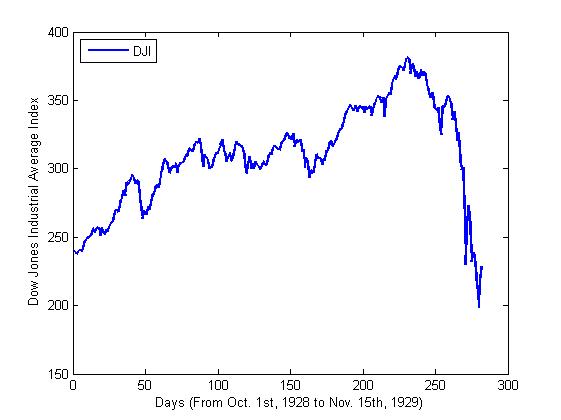
Figure
3- Index of SSEC (Apr. 19th, 1999-Oct. 15th,
2001)
Before predicting we did a simple preprocessing with the original
data. As unusually done in the economic analysis, we did a logarithmic
transformation to the data and then scale it into the range of [0, 1]. We
choose Gaussian Radial function as the kernel function in the experiment. For
each train set, we use the previous six days’ data to predict the seventh day’s
price. There are 74 sets of training data (i.e. 80 days’ market indices) that
is to say we will discover and memorize the sequence’s statistical law through
the previous 80 days’ data and predict the rest days’ indices in the period.
Here I make a comparison between the traditional Linear Regression (LR) method
and SVR. The result is shown in figure 2.4 The blue line represents the actual
index of the market and the red stars represent the output from the SVM. The
training error is 0.0061 and the testing error is 0.0078The black line represents the output of
from LR. of SVR0.00580.0047
The training error of LR is 0.0174 and the testing error is 0.0151. From Figure
4 we can see that the curve of SVR lies more close to the actual index curve
and it can capture more details of the actual index curve that the curve of LR.
What is more the trend of the curve is more delayed for the LR method which
means a serious problem when you use the method to make real decisions about
the transaction of the stock market.
Figure
4-experiment result
Sensitivity of the system to Parameters
As stated in [1], there is an absence of a structured method to
select the free parameters of SVMs, the generalization error with respect to
the delay of days and C are studied in my project. The dataset used is still
the same. Figure 5 illustrates the generalization error versus days of delay.
The blue color represents the error generated by SVR and the red color
represents the error generated by LR. The solid lines represent training error
and the dotted lines represent the testing error. Here we can see that the
training error of SVR decreases at first and increases then while the testing
error of SVR keeps decreasing. So we can find the best value for the choice of
days of day which is 6. Figure 6 illustrates the generalization error versus C.
From the figure we find that the generalization error is not influenced greatly
by C. There is not obvious increase of the error when C rises from 100 to 2000.
Figure
5 RMSE comparison of SVR and LR with respect to days of delay
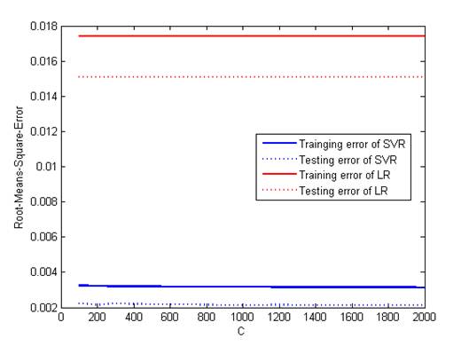
Figure
6 RMSE comparison of SVR and LR with respect to C
Conclusions
In this project I mainly apply SVM to predict the index of stock
market. It is shown that SVM is a promising method to for financial time series
forecasting. What is more the choice of the days of delay will have an impact
on the training and predicting procedure of the algorithm while the choice of
the constant C has nearly no impact on the performance of the algorithm.
Reference
[1] L. J. Cao and F. E. H. Tay, "Financial
forecasting using support vector machines", Neural Comput.
Applicat., vol. 10, no. 2, pp. 184-192, 2001.
[2] Vatsal H. Shah, “Machine Learning Techniques for Stock
Prediction”, http://www.vatsals.com/Essays/MachineLearningTechniquesforStockPrediction.pdf
[3] R. Choudhry and K. Garg, "A hybrid machine learning system for stock
market forecasting," Proceedings of World Academy of Science, Engineering
and Technology, vol.29, pp. 315-318, 2008.
[4]T. B. Trafalis and H. Ince. Support
vector machine for regression and applications to financial forecasting.
IJCNN2000, 348-353
[5] http://in.finance.yahoo.com/
[6]K Kim, Financial time series
forecasting using Support Vector Machines, Neurocomputing
55, May 2003, Pages 307-319.
[7]Wun-Hua
Chen and Jen-Ying Shih, Comparison of support-vector machines and back
propagation neural networks in forecasting the six major Asian stock markets,
Int. J. Electronic Fiance, Vol. 1, No. 1, 2006.
[8]. AJ Smola,
B. Scholkopf, A tutorial on support vector
regression, NeuroCOLT2 Tech. Report, NeuroCOLT, 1998.